e | Daniel's blog

What does e actually represent?

I’ve been using $e$ for years. Exponential growth and decay, compound interest, calculus especially, and statistics. But for some reason, only recently I asked myself what $e$ really means. What does it represent? There has to be some deep meaning behind it. But I struggled to find an intuitive explanation. Every video either told me its origin, its derivation, or its nifty uses.

If you’re like me, I encourage you to keep reading, or watch this video by FoolishChemist. It’s the first video that made $e$ click for me and is the basis for my own personal explanation below.

$e$ as we know it is $\approx2.718281828459045$ But, what does it represent?

Well we know what $\pi$ represents. Simple: the ratio of a circle’s circumference to its diameter. ($\pi$ also pops up in other areas)

alt text

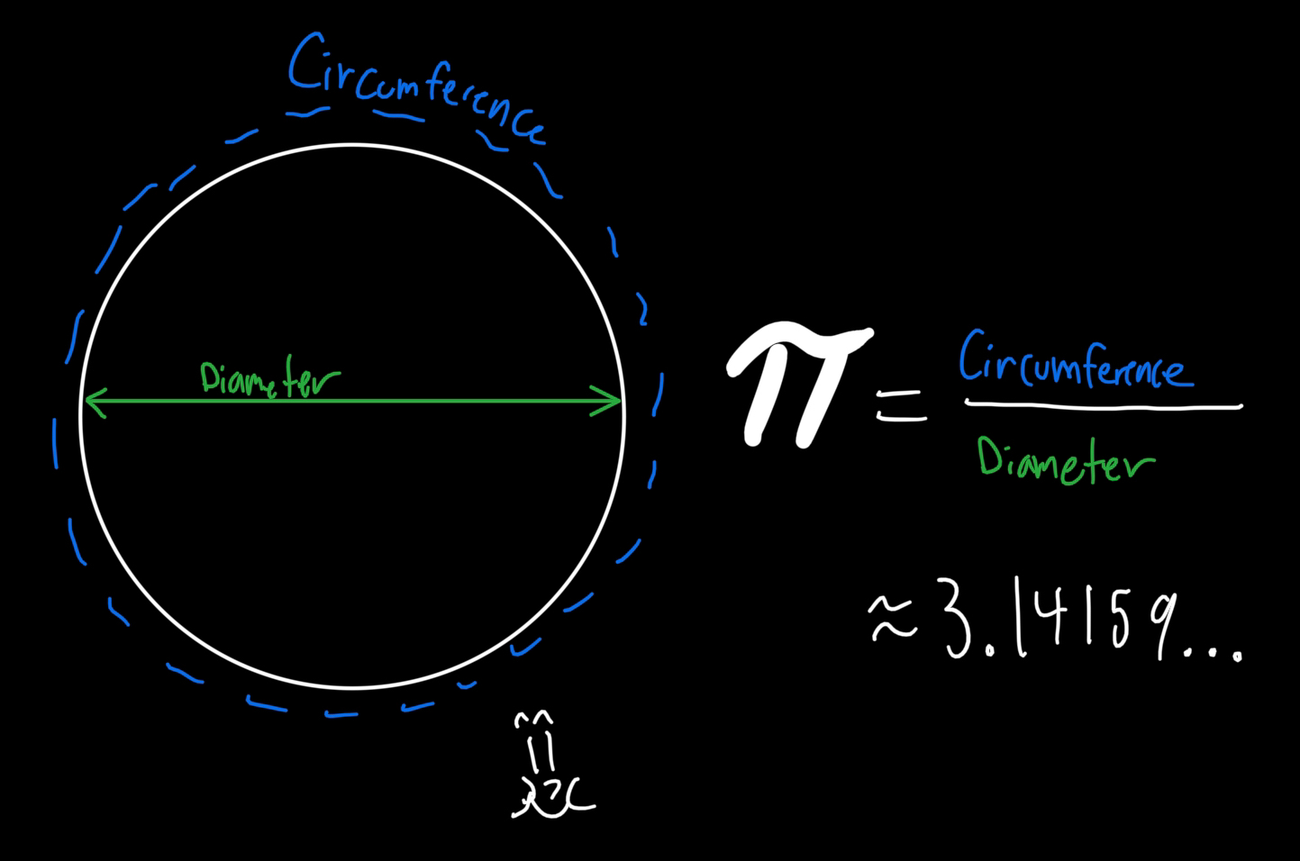
As far as I can tell it’s just a physical relationship between two things in our universe that we express numerically in base-10. $\pi$ could be expressed in base-3 ($\approx10.01021101$) just the same. Aliens will know the same value, maybe they’ll have a cooler name for it.

But there’s no intuitive one sentence explainer for $e$. Hopefully the one you read at the end of this blog is digestible.

Let’s begin

If you’ve done similar research, you’ve seen this derivation before, but roll with me a bit. Say I got $\$1$ in my savings account that offers $\bold{5\%}$ interest annually. How much do I have in that account after one year?

$1*1.05$ or $1(1 + 0.05) = \$1.05$
not too much money 😔

But what if… I ask my bank to do $\bold{2.5\%}$ interest semiannually? - So $2.5\%$ interest twice a year. Do I get more or less?

$1(1 + \frac{0.05}{2})^2 => 1(1.050625) = \$1.050625$
Boom! By taking split interest at a higher frequency, our money grows faster. Why?

How much our money grows is determined by our principal amount. In the first example, interest is applied only once to our principal $\$1$. But in the second example, interest is being applied here not just on our principal amount, but on the accrued interest as well, e.g. $(1*1.025)*1.025$. That’s why our money grows slightly faster.

If interest is applied onto itself, that’s called compound interest.

What if we keep splitting the interest and applying it more and more frequently? Does our money just keep growing?

Every month: $1(1 + \frac{0.05}{12})^{12} = \$1.051162$

Every day: $1(1 + \frac{0.05}{365})^{365} = \$1.051267$

Every second: $1(1 + \frac{0.05}{31536000})^{31536000} = \$1.051271$

The answer is no. There’s a limit, and I’m gonna skip past the calculus and tell you it’s precisely $\bold{1.051271}$. Why do we land on this number specifically? Like $\pi$, it just happens to be the number we derive from doing these exercises and formulas. Ok then… what is it exactly and what can we do with it?

Things to note

Interest applied at discrete points (e.g. once a year, twice a year) is an example of discrete self-referential growth.
Interest applied at infinite points, or continuously over a period, is called continuous self-referential growth.

A few times throughout this blog my language may seem ambiguous. Whenever I’m describing growth, I’m referring to self-referential growth. I also interchange continuous/natural growth.

Many things in nature are examples of continuous self-referential growth. A population of bacteria in a petri dish doesn’t double every few seconds in front of your eyes. It’s a smooth, continuous growth of bacteria. (In this case the bacterium are reproducing at different times fast enough for it to appear continuous)

To calculate a final amount for a discrete self-referential growth process (like how much money I have in my savings account at the end of the year), we just use a multiplicative factor
- $1*\bold{1.05}$ for $5\%$ per year (multiplicative factor is $1.05$)
- $1*\bold{1.050625}$ for $2.5\%$ semiannually
How do we calculate the final amount for continuous self-referential growth? Well we just calculated the multiplicative factor for $5\%$: $\bold{1.051271}$!
- This means that if our bacteria grow continuously at a rate of $5\%$ per hour, at the end of the hour we’ll have $1.051271$ times our bacteria.

Bingo! $\bold{1.051271}$, which we calculated above by taking the limit of discrete self-referential growth at $5\%$, is the multiplicative factor for continuous self-referential growth at a rate of $\bold{5\%}$.

Uses of $d$

So now we have this number: $1.051271$. Let’s call it $\bold{d}$. What can we do with $d$? Well here’s some cool things.

If my bank account gives me $5.1271\%$ yearly interest, the multiplicative factor for that discrete growth is equivalent to the multiplicative factor of continuous growth at $5\%$ ($d$).
$1.051271 = 1.051271$

Conversely, if my bank account gives me $5\%$ yearly interest (applied once a year), I can calculate the interest rate (growth rate) of an equivalent compounding account (continuous). We can calculate it using $d$.

We can use this equation: $d^x = 1.05$ where $d^x$ is the multiplicative factor of some continuous growth percentage.
To calculate this, we can use log. $x = \log_d{1.05}$. The log side of the equation is asking “to what exponent do we need for $d$ to produce $1.05$. Well we know $d$, so plugging it into our calculator we get: $\log_{1.051271}{1.05} = .9758$ $d^{.9758} = 1.05$
What does this tell us about the equivalent rate of continuous self-growth? Well, it’s
$.9758 * 5\%$ or $4.879\%$
This tells me that $5\%$ yearly interest on my account is equivalent to my money growing at $4.879\%$ continuously over the year.

ANY discrete self-referential growth process can be expressed in powers of $d$!

Woah woah waoh… how is our exponent $.9758$ also the scaling factor for our $5\%$ continuous self-referential growth rate? Why does this whole exponent thing work? Well, here’s an easier example.

If we’re trying to get the multiplicative factor of continuous growth at $10\%$ for the same period, we can just apply the multiplicative factor for continuous growth at $5\%$ ($d$) twice.
I have $\$1$ to start. $1*1.051271*1.051271 = \$1.10517$
Our money grows $5\%$ to start, then it grows $5\%$ more! $10\%$! But it’s the same thing as squaring the number!
$1*(1.051271)^2 = 1.10517$. So if our exponent is $2$, we’re getting the multiplicative factor of $2 * 5\%$ or $10\%$ continuous self-referential growth!

Wait… do you see what we just did? Given our multiplicative factor for continuous self-referential growth at $5\%$ $d$, we raised it to a power of $2$ to find the multiplicative factor for continuous self-referential growth at $10\%$!! $(2 * 5\%)$. So this means…

ANY continuous self-referential growth process can also be expressed in powers of $d$!

Great, so looks like $d$ has some cool features.

It’s the multiplicative factor for continuous self-referential growth at a rate of $5\%$. (boring 🥱)
We can use $d$ to describe any discrete/continuous self-referential growth process just using exponents. (wow!!!)

Let’s test it out.

What if I want to find the multiplicative factor for my population that grows at $40\%$ continuously?

Well, since $d$ is the multiplicative factor for continuous self-referential growth at $5\%$, we just need to exponentiate it to $8$, since $8 * 5\%$ is $40\%$. We’re applying $5\%$ continuous growth $8$ times.

\[d^{8} => 1.051271^{8} = 1.49182\]

Let’s verify this!

\[\lim_{n \to \infty} 1(1 + \frac{.40}{n})^n\]

(Same equation we used to find the multiplicative factor for $5\%$ at the beginning.)

We can approximate the limit by using $n = 100000$

\[1(1 + \frac{.40}{100000})^{100000} \approx 1.49182\]

Same answer!

Another example.

Say my savings account applies $25\%$ interest annually (pretty sweet). What is an equivalent continuous growth rate that I can express in terms of $d$?

Well the multiplicative factor for $25\%$ annual interest is simply $1.25$. So I can use $log$ to compute the exponent for $d$.

\[d^x = 1.25\] \[\log_{d}{1.25} = x\] \[\log_{1.051271}{1.25} = 4.463\] \[4.463 * 5\% = 22.314\%\]

The answer is a continuous self-referential growth rate of $22.314\%$, or $d^{4.463}$.

Now what?

Isn’t it a bit frustrating that we need to calculate everything relative to the $5\%$ multiplicative factor? For the $40\%$ example. we had to exponentiate to $8$. In the second example, we had to multiply our exponent by $5\%$ to find the rate. Is there a better way?

What if… $d$ wasn’t the multiplicative factor for $5\%$ continuous self-referential growth, but for $100\%$. Would that fix it? Well let’s see…

In the $40\%$ example, our exponent would just be $.4$ instead of $8$ (remember the exponent/scaling rule) - which is the exact rate we’re trying to calculate. Pretty intuitive right?

In the savings account example, our exponent (answer to the log function) would also be the exact equivalent continuous rate. We wouldn’t have to scale $5\%$ to find that rate. Huh.

So what’s this fancy $100\%$ multiplicative factor then? You might be getting it now…

Deriving a new number

We can just approximate this $100\%$ multiplicative factor for continuous growth using the same equation for $40\%$ or $5\%$. (We can easily use the $5\%$ multiplicative factor but I’m going back to first steps). Instead of $.4$ I’m using $1.0$ to denote a $100\%$ growth rate.

\[\lim_{n \to \infty} 1(1 + \frac{1.0}{n})^n\]

Approximation:

\[1(1 + \frac{1.0}{100000})^{100000} \approx 2.7183\]

Looks familiar? It’s $\bold{e}$!

\[e \approx 2.718281828\]

We can even calculate it using our constant $d$! $20*5\% = 100\%$

\[d^{20} = e\] \[1.051271^{20} \approx 2.7183\]

$e$ is the multiplicative factor of continuous self-referential growth at a rate of 100%.

Testing with e

What’s the multiplicative factor for continuous self-referential growth at a rate of $40\%$? Simple.

\[e^{.40} = x\] \[2.71828^{.40} \approx 1.49182\]

That’s what we got before! What about the bank account example with discrete growth at $25\%$? What’s the equivalent continuous rate?

\[\log_{e}{1.25} = x\] \[\log_{2.71828}{1.25} \approx .22314\]

$.22314$ is the exact rate we got before! And we don’t need to scale anything.

Calculus references

Let’s take a closer look at the log function we just used.

\[\log_{e}x\]

It’s asking to what continuous rate yields the growth factor $x$. But we see this function elsewhere:

\[\ln{x}\]

The natural logarithm, $\ln{x}$, is just $\log_{e}x$! The one we’ve been using! It describes the natural rate of change given a growth factor. It’s the inverse of $e^{x}$. So why is the derivative of $\ln{x} = \frac{1}{x}$? Well, think about it like this. What is $x$? It’s the growth factor we’re using to find an equivalent rate of natural change. For now we can use the example of discrete growth applied once per period. Then our discrete rate is just that factor. $25\% = 1.25, 50\% = 1.5$. How does the natural rate grow? $\ln{1.25} = .223$, $\ln{1.5} = .405$, or $22.3\%$ and $40.5\%$. The difference in natural to discrete growth rate is increasing $(25-22.3, 50-40.5)$. This makes sense because natural growth is more powerful, and the higher rate we give it for a period, the less it needs to catch up to discrete growth, so to speak. So we express this relationship in terms of the inverse of the input $(1/x)$, since our output never decreases but it decays as $x$ (discrete growth rate) increases.

Now let’s take a look at this:

\[e^{x}\]

The equation asks, given a growth rate $x$, what’s the multiplicative factor for continuous self-referential growth?
Well then, what’s the derivative of $e^x$? We’re looking for the instantaneous rate of change of the function, or how much $e^x$ changes given a small change in $x$. As a reminder, $x$ in this function is a growth rate, and our output is the multiplicative factor for that natural growth rate. Let’s try some things out.
$e^{1} \approx 2.718$
$e^{2} \approx 7.389$
$e^{3} \approx 20.09$
If you remember the exponent/scaling rule here, setting $e$ to $2, 3, .5, etc.$ is just applying that multiplicative factor $x$ times to get our answer. The multiplicative factor for a natural rate of $200\%$ is just applying the $100\%$ factor twice for a rate of $2.0$: $e*e$ or $e^2 = 7.389$. So our output (multiplicative factor) is proportional to, no, exactly however many times we apply $e$, which is determined by $x$ right? But that’s not what the derivative is asking. How much does our output change given a change in $x$? Well our output is changing… $e^x$ times for every $x$. What? Is that right? For every $2$ $x$, our output is changing $e^{2}$ or $7.389$? What about $e^4$? $e^4 \approx 54.60$, which is $7.389$ times more than $e^{2}$. It makes sense because we’re we’re applying $e$ $4$ times, or $e^{2}$ twice. For every $x$, we scale our factor by another $e$, so our derivative (instantaneous rate of change) is literally $e^x$!

Let’s verify this using the classic derivative formula.

\[\frac{d}{dx}e^x=\lim_{h \to 0}\frac{f(x+h) - f(x)}{h}\] \[\frac{d}{dx}e^x=\lim_{h \to 0}\frac{e^{x+h} - e^x}{h}\] \[\frac{d}{dx}e^x=\lim_{h \to 0}\frac{e^{x}e^{h} - e^x}{h}\] \[\frac{d}{dx}e^x=e^x\lim_{h \to 0}\frac{e^{h} - 1}{h}\]

We can approximate the limit:

\[\frac{d}{dx}e^x=e^x\frac{e^{.0000001} - 1}{.0000001}\] \[\frac{e^{.0000001} - 1}{.0000001} \approx 1\] \[\frac{d}{dx}e^x=e^x*1 = e^x\]

Verified.

Why do we use e?

$\frac{d}{dx}e^x=e^x$ This is one of the most important properties of $e$. If we try to differentiate the function $2^x$, we don’t get a nice limit.

\[\frac{2^{.0000001} - 1}{.0000001} \approx .6931\] \[\frac{d}{dx}2^x=2^x*.6931 = (.6931)(2^x)\]

We get a nasty constant on this derivative. What about on our other constant, $d$?

\[\frac{1.051271^{.0000001} - 1}{.0000001} = .05\] \[\frac{d}{dx}d^x=d^x*.05 = (.05)(d^x)\]

Ah, interesting… remember $d$ is our multiplicative factor for continuous self-referential growth at a rate of $5\%$. That $.05$ showing up isn’t a coincidence.

What’s happening here? You can think of taking the derivative as inspecting the natural growth of a function at an instant. I say natural because in nature, growth is continuous. At any point, there is an instantaneous growth rate of a population, of temperature, etc., that is affected by its current state. It’s hard to take the derivative of a discrete growth function. It’s like asking how much is my money growing per second if interest is applied only once at the end of the year. Well, in reality, the money doesn’t increase until interest is applied at the end of the year, but what you can do is pretend it’s a continuous growth function with $e$ using $ln$ like I showed earlier.

So why does the derivative of $e^x$ equal itself but swapping out other numbers for $e$ gives us nasty constants? It’s because $e$ is standardized to $1$. I’ll show you.

$2^x$ is similar to $e^x$. But we know $e$ is the multiplicative factor for a $100\%$ continuous growth rate. If we pretend $2$ is a multiplicative factor for some continuous growth rate, we have no idea what that growth rate is. But, lucky for us, it popped up: $\frac{d}{dx}2^x=2^x*.6931 = (.6931)(2^x)$ $2$ would be a multiplicative factor for a continuous growth rate of $69.31...\%$ It’s ugly, but just like $e$, $2$ can be used to express discrete and continuous growth processes, but everything must be scaled relative to the irrational $.6931...$, which no one in their right mind will want to do. But this gives us a little more clarification why $e$ is used so prolifically.

Let’s say I have a population $P$. My population grows at a continuous rate of $r$ per period $t$. In this example my population is $P_0 = 50$. My rate is $r = .14$, and I check after $t = 2$ periods. The equation would look like this. We’re using $e$ to find the multiplicative factor for continuous growth at a $(.14 * 2)\%$ rate to then scale our initial population with.

\[P(t) = P_0e^{rt}\] \[P(t) = 50e^{.14*2}\] \[66.16 = 50e^{.14*2}\]

But google the equation for continuous compounding interest. It’s the exact. same. thing.

\[P(t) = P_0e^{rt}\]

But imagine now if we used $2$ instead of $e$.

\[P(t) = 50(2)^{.14*2}\]

Now we need to standardize our exponent to the .6931 scale since 2 is the factor for $69.31...\%$ growth rate.

\[P(t) = 50(2)^{.28/.6931}\] \[P(t) = 50(2)^{.40398}\] \[P(t) = 50(1.3232)\] \[66.16 = 50(1.3232)\]

See, it worked just the same. But it was a whole lot uglier, which is why we use $e$ instead of $2$. This follows in many other equations that use $e$.

Exponential growth and decay

\[N(t) = N_0e^{rt}\]

Continuous compounding (finance)

\[P(t) = P_0e^{rt}\]

Poisson distribution (statistics)

\[P(k;\lambda) = \frac{\lambda^ke^{-\lambda}}{k!}\]

Normal distribution (statistics)

\[y = \frac{1}{\sigma\sqrt{2\pi}}{e^{-\frac{(x-\mu)^2}{2\sigma^2}}}\]

Fourier transform

\[f(x) = \int_{-\infty}^{\infty}F(k)e^{2\pi ikx}dk\]

And many others…

Remember this: the multiplicative factors of continuous self-referential growth rates follow the same universal pattern, but $e$ is the most convenient to use (standardized to 1, derivative, natural log).

Conclusion

$e$ is the multiplicative factor for continuous self-referential growth at a rate of 100%.

That’s the sentence. $e$ is just a word we plucked from the vocabulary of natural growth because it’s the easiest word to use. Not only does it describe natural growth, but we use it in our equations, derivations, calculus, logarithms, etc. to find other continuous self-referential growth factors. It makes our lives a bit simpler and the math a bit quicker.

If this atrociously long blog helped you understand $e$ just a little bit more, then I accomplished my goal. I hope you enjoyed reading!

e